Create ggplot plots in a loop. � ggloop • ggloop

ggloop() mimics ggplot() by accepting both a data frame and mappings, returning a plot - or plots in this case. The main difference is that ggloop() accepts vectors for aesthetics and returns a list or nested list of ggplot plots.

ggloop(data, mappings = aes_loop(), remap_xy = TRUE, remap_dots = FALSE,
  gg_obs = TRUE, ..., environment = parent.frame())

Arguments

data: Default dataset to use for plot. Must be a data frame and can be only one data frame.
mappings: List of aesthetic mappings to use for plots. Works like mapping from ggplot().
remap_xy: Remapping behavior of the x and y vectors specified in aes_loop(). See details below for more on remapping behavior.
remap_dots: Remapping behavior of the ... vectors specified in aes_loop(). See details below for more on remapping behavior.
gg_obs: Logical. Specifies whether to return plots or the list (or nested list) of aesthetics used to make such a plots.
...: Other arguments. Similar to ggplot()'s ....
environment: An environment and only one environment (cannot be a vector). Similar to ggplot()'s environment.

Details

ggloop() makes use of aes_loop, which is meant to mimic aes from ggplot2. Because of this, the remapping arguments are supplied to ggloop instead of aes_loop().

The first remapping argument, remap_xy can take three values:

TRUE = The default behavior. All unqiue combinations of x and y are generated. This means that if a variable (i.e. mpg) is supplied in both x and y, then no mapping will have x and y variables that are the same (i.e. x -> mpg; y -> mpg will not ever happen). Likewise, no unordered pair duplicates will happen (i.e. x -> mpg; y -> cyl and x -> cyl; y -> mpg will be treated the same).
FALSE = If x and y vectors are not the same length, then the shorter of the two will be recycled. Recycling is similar to mapply()'s recycling.
NA = If x and y vectors are not the same length, then the shorter of the two will have NA assigned to the missing elements. These are meant to act as placeholders during the wrangling operations (extracting and grouping the aesthetics), and will be taken out before the final list of mappings is sent to ggloop().

Examples

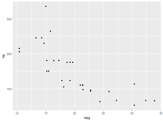
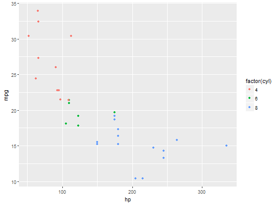
# 1. Return all possible x-y combinations.
plots <- ggloop(data = mtcars,
                mappings = aes_loop(x = mpg:carb, y = mpg:carb))
names(plots)
#>  [1] "x.mpg_y.cyl"   "x.mpg_y.disp"  "x.mpg_y.hp"    "x.mpg_y.drat" 
#>  [5] "x.mpg_y.wt"    "x.mpg_y.qsec"  "x.mpg_y.vs"    "x.mpg_y.am"   
#>  [9] "x.mpg_y.gear"  "x.mpg_y.carb"  "x.cyl_y.disp"  "x.cyl_y.hp"   
#> [13] "x.cyl_y.drat"  "x.cyl_y.wt"    "x.cyl_y.qsec"  "x.cyl_y.vs"   
#> [17] "x.cyl_y.am"    "x.cyl_y.gear"  "x.cyl_y.carb"  "x.disp_y.hp"  
#> [21] "x.disp_y.drat" "x.disp_y.wt"   "x.disp_y.qsec" "x.disp_y.vs"  
#> [25] "x.disp_y.am"   "x.disp_y.gear" "x.disp_y.carb" "x.hp_y.drat"  
#> [29] "x.hp_y.wt"     "x.hp_y.qsec"   "x.hp_y.vs"     "x.hp_y.am"    
#> [33] "x.hp_y.gear"   "x.hp_y.carb"   "x.drat_y.wt"   "x.drat_y.qsec"
#> [37] "x.drat_y.vs"   "x.drat_y.am"   "x.drat_y.gear" "x.drat_y.carb"
#> [41] "x.wt_y.qsec"   "x.wt_y.vs"     "x.wt_y.am"     "x.wt_y.gear"  
#> [45] "x.wt_y.carb"   "x.qsec_y.vs"   "x.qsec_y.am"   "x.qsec_y.gear"
#> [49] "x.qsec_y.carb" "x.vs_y.am"     "x.vs_y.gear"   "x.vs_y.carb"  
#> [53] "x.am_y.gear"   "x.am_y.carb"   "x.gear_y.carb"
# [1] "x.mpg_y.cyl"   "x.mpg_y.disp"  "x.mpg_y.hp"    "x.mpg_y.drat"
# [5] "x.mpg_y.wt"    "x.mpg_y.qsec"  "x.mpg_y.vs"    "x.mpg_y.am"
# [9] "x.mpg_y.gear"  "x.mpg_y.carb"  "x.cyl_y.disp"  "x.cyl_y.hp"
# [13] "x.cyl_y.drat"  "x.cyl_y.wt"    "x.cyl_y.qsec"  "x.cyl_y.vs"
# [17] "x.cyl_y.am"    "x.cyl_y.gear"  "x.cyl_y.carb"  "x.disp_y.hp"
# [21] "x.disp_y.drat" "x.disp_y.wt"   "x.disp_y.qsec" "x.disp_y.vs"
# [25] "x.disp_y.am"   "x.disp_y.gear" "x.disp_y.carb" "x.hp_y.drat"
# [29] "x.hp_y.wt"     "x.hp_y.qsec"   "x.hp_y.vs"     "x.hp_y.am"
# [33] "x.hp_y.gear"   "x.hp_y.carb"   "x.drat_y.wt"   "x.drat_y.qsec"
# [37] "x.drat_y.vs"   "x.drat_y.am"   "x.drat_y.gear" "x.drat_y.carb"
# [41] "x.wt_y.qsec"   "x.wt_y.vs"     "x.wt_y.am"     "x.wt_y.gear"
# [45] "x.wt_y.carb"   "x.qsec_y.vs"   "x.qsec_y.am"   "x.qsec_y.gear"
# [49] "x.qsec_y.carb" "x.vs_y.am"     "x.vs_y.gear"   "x.vs_y.carb"
# [53] "x.am_y.gear"   "x.am_y.carb"   "x.gear_y.carb"

plots$x.mpg_y.hp + ggplot2::geom_point()

# 2. Add an additional aesthetic (facet) to plots.
plots2 <- ggloop(data = mtcars,
                 mappings = aes_loop(
                                     x = c(disp, hp, wt),
                                     y = mpg,
                                     color = factor(cyl)))
sapply(plots2, names)
#>      color.factor(cyl)
#> [1,] "x.disp_y.mpg"   
#> [2,] "x.hp_y.mpg"     
#> [3,] "x.wt_y.mpg"     
#      color.factor(cyl)
# [1,] "x.disp_y.mpg"
# [2,] "x.hp_y.mpg"
# [3,] "x.wt_y.mpg"

plots2$`color.factor(cyl)`$x.hp_y.mpg + ggplot2::geom_point()

# A look at remap_xy's other two behaviors:
# 3. remap_xy = NA
#    The longer vector will go "unpaired" after the shorter vector
#    runs out of elements.
plots3 <- ggloop(data = mtcars,
                 mappings = aes_loop(x = c(mpg/disp, mpg/hp, mpg/cyl, mpg/gear),
                                     y = c(hp, disp)),
                 remap_xy = NA)
names(plots3)
#> [1] "x.mpg/disp_y.hp" "x.mpg/hp_y.disp" "x.mpg/cyl"       "x.mpg/gear"     
# [1] "x.mpg/disp_y.hp" "x.mpg/hp_y.disp" "x.mpg/cyl"       "x.mpg/gear"

# 4. remap_xy = FALSE
#    The longer vector will be "paired" with the shorter vector using
#    recycling (similar to R's internal recycling, i.e. mapply()).
plots4 <- ggloop(data = mtcars,
                 mappings = aes_loop(x = c(mpg/disp, mpg/hp, mpg/cyl, mpg/gear),
                                     y = c(hp, disp)),
                 remap_xy = FALSE)
sapply(plots4, names)
#>       x.mpg/disp_y.hp x.mpg/hp_y.disp x.mpg/cyl_y.hp x.mpg/gear_y.disp
#>  [1,] "data"          "data"          "data"         "data"           
#>  [2,] "layers"        "layers"        "layers"       "layers"         
#>  [3,] "scales"        "scales"        "scales"       "scales"         
#>  [4,] "mapping"       "mapping"       "mapping"      "mapping"        
#>  [5,] "theme"         "theme"         "theme"        "theme"          
#>  [6,] "coordinates"   "coordinates"   "coordinates"  "coordinates"    
#>  [7,] "facet"         "facet"         "facet"        "facet"          
#>  [8,] "plot_env"      "plot_env"      "plot_env"     "plot_env"       
#>  [9,] "labels"        "labels"        "labels"       "labels"         
# [1] "x.mpg/disp_y.hp"   "x.mpg/hp_y.disp"   "x.mpg/cyl_y.hp"    "x.mpg/gear_y.disp"

Create ggplot plots in a loop.

Arguments

Details

Examples

Contents